
The area model is a powerful visual tool for organizing multi-digit multiplication. It is build on the premise that the area of a rectangle is the length of the rectangle times the width. Thus, when we set up multiplication in an area model, we start with a rectangle and label two adjacent sides with the two factors (the numbers being multiplied together) and find the area of the rectangle in order to know what the product (the result of multiplication) is.
If you’d like to know more about how and why the area model works, check out any of the following:
- Area Model Math (blog post)
- What Does an Area Model Represent? (blog post)
- What is the Area Model? (video)
- Why Does the Area Model Work? (video)
This post was originally published on mathteacherbarbie.com. If you are reading it somewhere else, you are reading a stolen copy.
How to set up Area Model Multiplication
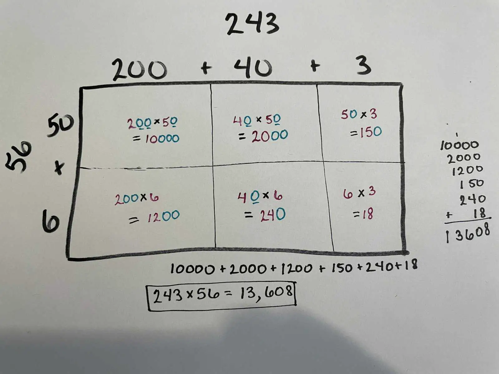
Our main example, $243 \times 56$, plays to the strengths of the area model. Namely, the area model works best when multiplying two-or-three digit numbers together. If you’d like to see a second example worked out, check out my video Using the Area Model to Multiply Larger Numbers.
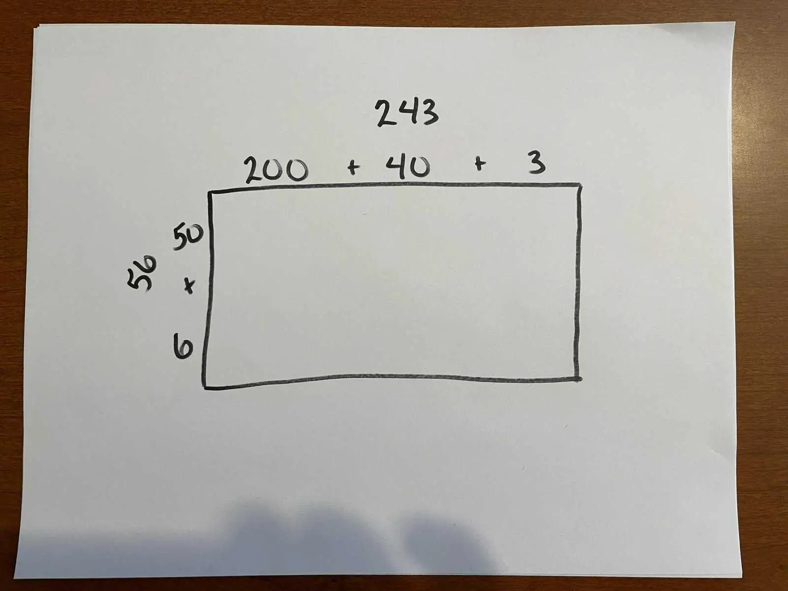
First, sketch out a rectangle. Then label the longer edge with the bigger number, decomposed into its place values, in this case, $243=200+40+3$. (It doesn’t actually matter which side is labelled with which number, but our brains tend to like it better if the longer side goes with the bigger number.) Label the shorter edge with the smaller number, decomposed into its place values, in this case, $56=50+6$.
Now break your larger rectangle into smaller ones along the $+$ signs of the decomposed numbers:
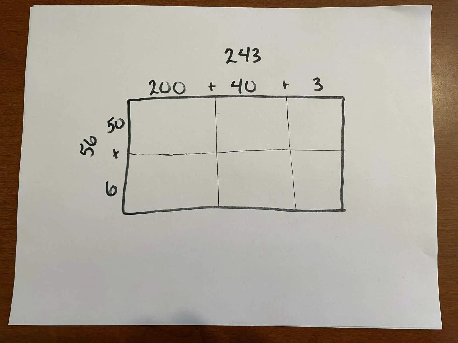
Now you’re all set up to multiply using the area model!
How to perform area model multiplication
If you know your multiplication facts well, the setup might just be the hardest part. The remaining steps are
- Find the area of each smaller rectangle by multiplying
- Add all the smaller areas together
- Report out the answer
Step 1: Find the area of each smaller rectangle by multiplying.
Rectangle by rectangle, move through the diagram, multiplying the number directly above by the number directly to the side. Write each result in the corresponding small box.
Step 2: Add all the smaller areas together.
Add together all of the products (the results of multiplying) from Step 1. Notice all the zeros! These happened because we split (or regrouped) each original factor (number being multiplied) into its place values. These zeros can make adding even a long list of numbers really easy!
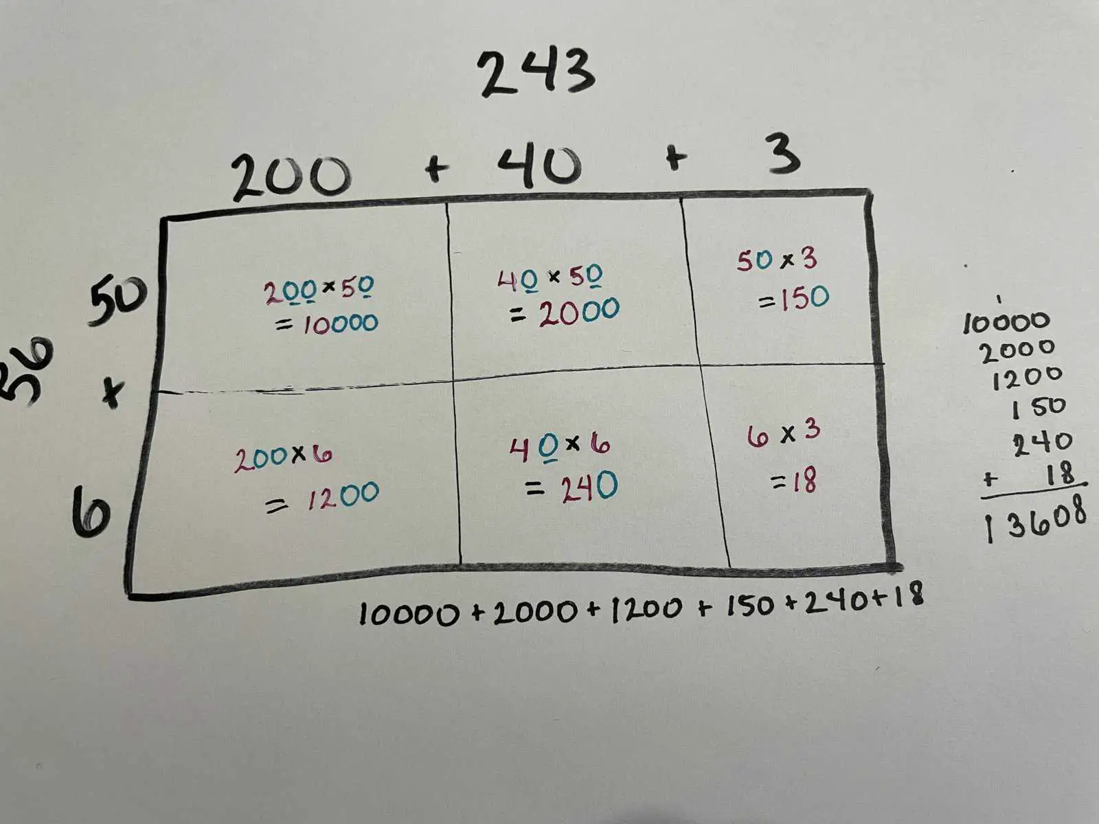
Step 3: Report out the answer.
Don’t forget the last step! Always make sure you finish by directly answering the question that was originally asked.
How the area model compares to traditional vertical multiplication
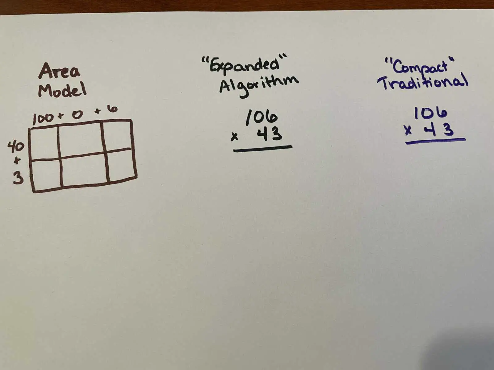
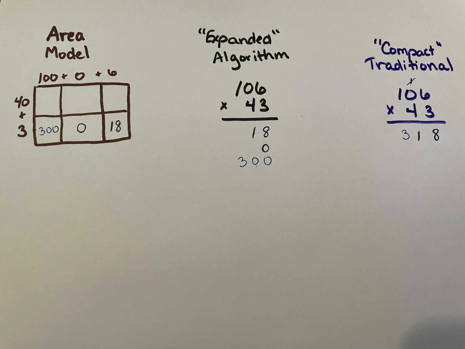
Turns out, the area model isn’t so much a “new” strategy as simply a different way of organizing the same information and procedure as the “traditional” algorithm. To demonstrate this, I’ll show a new problem there ways: using an area model on the left, using the traditional algorithm in its most compact form on the right, and using an expanded (less compact) version of the traditional algorithm in the middle. Let’s use for our example $106 \times 43$.
First, we set up each variation of our work. As I mentioned above, they’re all going to show the same work, the same steps, and the same information, just in different ways of organizing it.
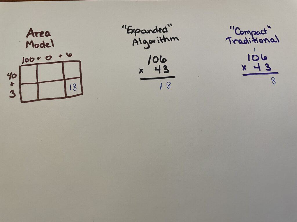
In each variation, let’s start with $6 \times 3$. The area model can be done in any order. Turns out the “expanded algorithm” will also work in any order, but we have a very prescribed order of doing the traditional “compact” algorithm for long multiplication. So we’ll follow that order. In the area model, we simply write the $18$ (since $6 \times 3=18$) in the appropriate box. In the expanded algorithm, since 18 is 1 ten and 8 ones, we write a 1 in the tens place and an 8 in the ones place. In the traditional algorithm, for the same reason, we write an 8 in the ones place below the line, and we carry (or regroup) the 1 up above the tens place to add it in later.
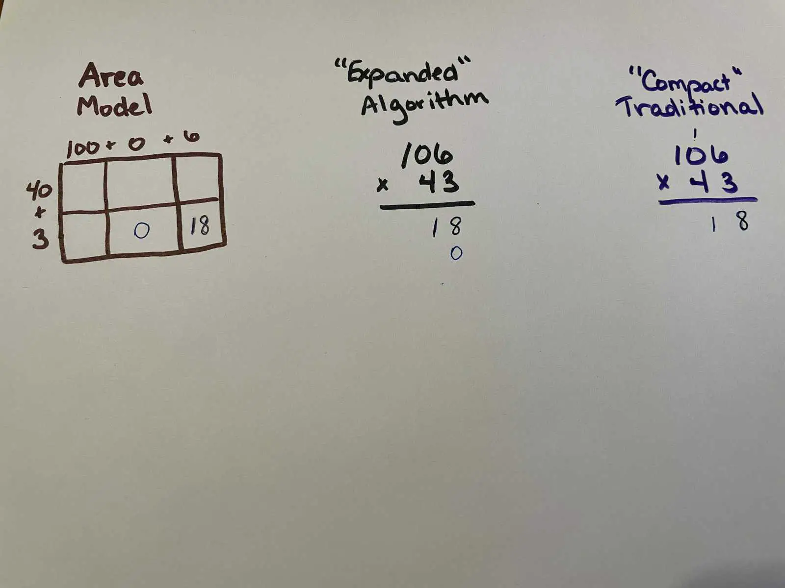
Next up is the $0 \times 3=0$ part. In the first two models, that shows up as a zero. However, in the traditional “compact” model, we have to remember to add the carried one, so we get $(0 \times 3)+1=1$ instead of the zero.
Next, the $1 \times 3$, which is really $100 \times 3=300$ since the 1 is in the hundreds place. We also cross off that “carried” one since we’ve used it now.
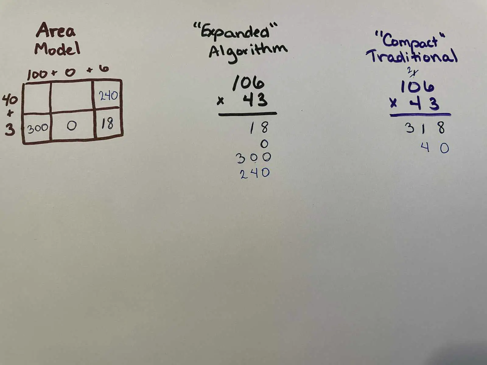
Next we move to the 4, which is really 40 since it’s in the tens place. To represent the “40”-ness in the traditional algorithm, we place a zero placeholder under the 8 (or maybe you learned to leave it as an open space). The other two methods both show and use 40 rather than a shortcut placeholder. $40 \times 6=240$. To keep the traditional algorithm compact (paper used to be expensive!), we carry the 2 up above the tens place again.
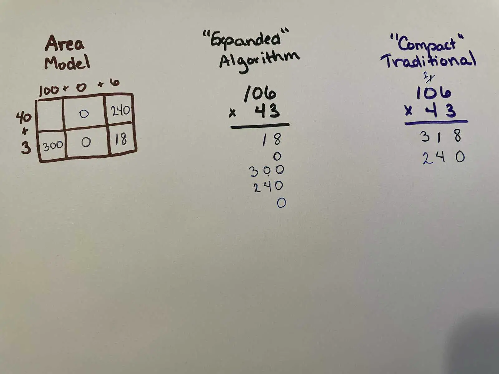
Next, $40 \times 0=0$. But don’t forget to add the carried 2 in the traditional compact algorithm!
Almost done with the multiplication part! Finally, the $40 \times 100=4000$.
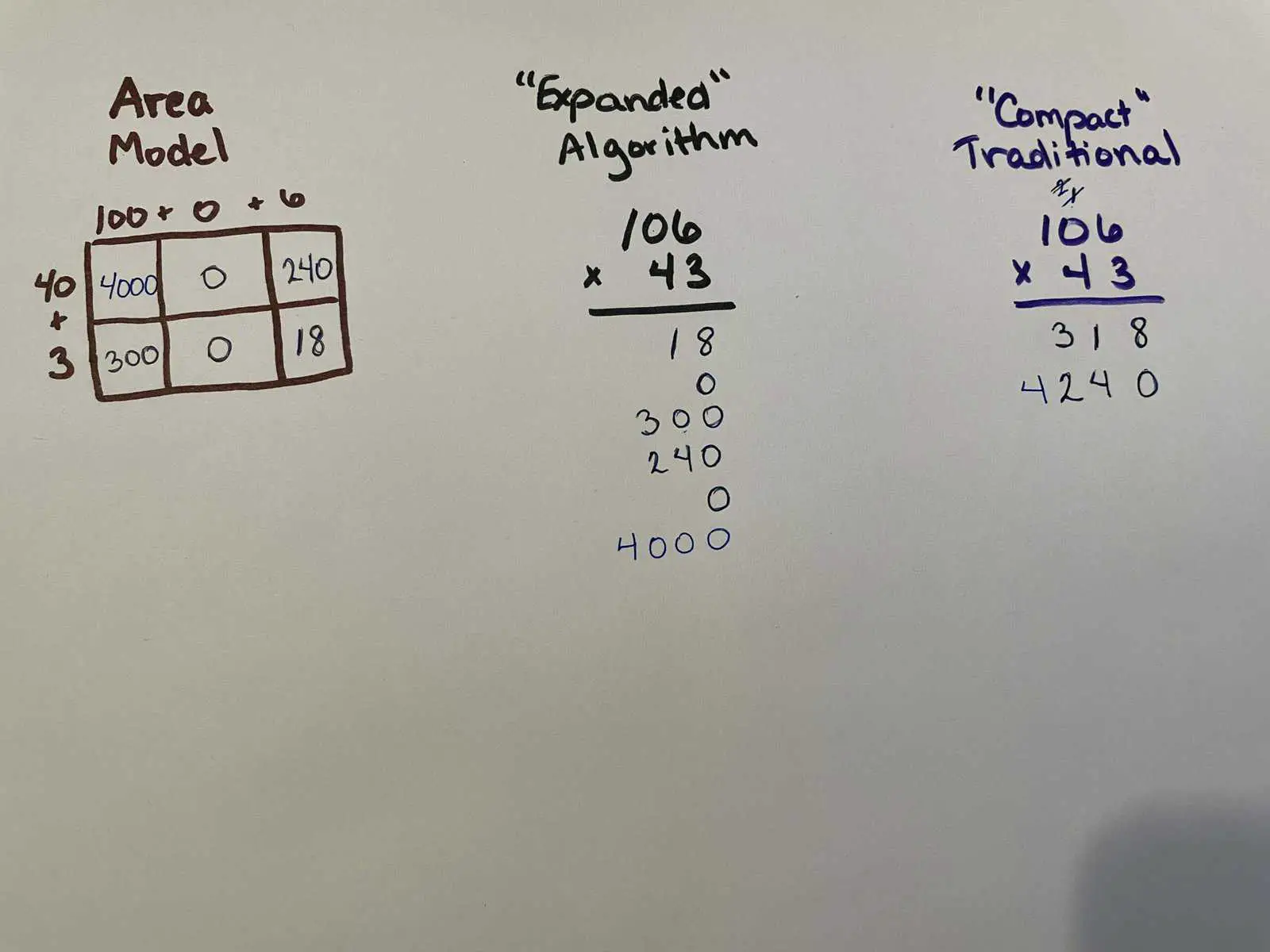
Finally, the next-to-last step in all three: Adding. And the last step: explicitly stating the solution.
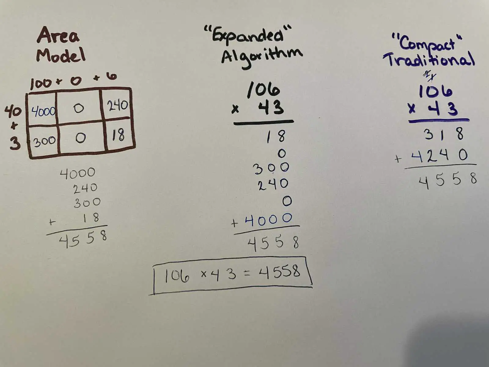
The traditional “compact” method’s main advantage is taking up less space. There’s a level of understanding and numeracy that the other two encourage. I find them easier to interpret and follow than the traditional algorithm. However, we can see how the traditional algorithm may have shown its advantage when space and speed were priorities. It is certainly the most space-saving.
To see another example comparing the area model to the traditional algorithm, check out my video Comparing Area Model to Traditional Algorithm.
You’ve Got This!